

In this article we're going to discuss several applications of classification-based machine learning in finance.
First, we'll start with a quick introduction to machine learning and how it fits into the quant workflow, and then we'll move on to several example projects.
The topics we'll cover include:
- Brief Introduction to Machine Learning
- Model Selection & the Quant Workflow
- Review of Logistic Regression
- Classification-Based Machine Learning
- Predicting the Next Day's Return
- Global Stock Selection with 14 Alpha Factors
The following guide is based on a course on Classification-Based Machine Learning in Finance by Andrew Ng and the code for this course can be found on Github here.
1. Brief Introduction to Machine Learning
Many hedge fund managers have moved beyond traditional investment strategies and into quantitative strategies in the search of alpha over the last 20 years.
In the last 5-10 years, we've seen a Big Data revolution that is characterized by 3 major trends:
- Massive increases in data
- Access to low-cost computing and data storage
- Advances in machine and deep learning
Let's quickly review the three main paradigms in machine learning: supervised learning, unsupervised learning, and reinforcement learning.
Supervised Learning
With supervised learning, we infer a function by using labeled training data.
The two subcategories of supervised learning are:
- Regression-based: these deal with continuous values, such as price, R2, etc.
- Classification-based: these deal with classes, such as 0 or 1, yes or no, etc.
Unsupervised Learning
With unsupervised learning we don't have any labels in our data, instead, the algorithm is trying to find structure in the data.
Common structures that unsupervised learning is used for include:
- Clustering
- Dimensionality reduction
Reinforcement Learning
Reinforcement learning is concerned with how software agents should act in an uncertain environment.
The goal of reinforcement learning is for the agent to learn how to operate in its environment and maximize its cumulative reward.
Check out these articles on reinforcement learning if you want to learn more about the subject.
Deep Learning
Deep learning is part of the broader family of machine learning is makes use of artificial neural networks.
Deep learning can be applied to all three learning paradigms: supervised learning, unsupervised learning, and reinforcement learning.
Subcategories in deep learning include:
- Artificial neural networks (ANNs)
- Convolutional Neural Networks (CNNs)
- Recurrent Neural Networks (RNNs)
Machine Learning Project Checklist
The following machine learning project checklist is from the textbook: Hands-On Machine Learning with Scikit-Learn & TensorFlow. The author defines 8 main steps to complete a machine learning project:
- Frame the problem and look at the big picture
- Collect the data
- Explore the data to gain insights into structure, values, and so on
- Prepare the data for machine learning
- Explore different machine learning models and short-list the top performing ones
- Fine-tune the models and combine them into a solution
- Present the solution
- Launch, monitor, and maintain the system
Let's now discuss how you actually choose the best model and how to assess it's performance.
Stay up to date with AI
2. Model Selection & the Quant Workflow
In supervised learning, we generally split our data into training sets and testing sets.
We also tune the model's hyperparameters ourselves as this is typically not directly learned by the model.
There are several approaches to optimizing a model's hyperparameters, and one of the most common is called grid search.
Model Selection
There are a few concepts to cover whenever you look at machine learning models.
Bias-Variance Tradeoff
The first is the bias-variance tradeoff, which is:
the property of a set of predictive models whereby models with a lower bias in parameter estimation have a higher variance of the parameter estimates across samples, and vice versa.
The bias is an error that arises from assumptions in the learning algorithm.
The variance is an error from sensitivity to small fluctuations in the training set.
Model Evaluation
In terms of model evaluation, a few methods we can use include:
- Mean absolute error (regression)
- Mean squared error (regression)
- Accuracy (classification)
- Log loss (classification)
- Adjusted rand score (clustering)
Validation Curve
We know that we need a scoring function to validate our model.
To do this we have a training score (which uses the training set) and a validation score (which uses the testing set).
From the scikit-learn documentation:
If the training score and the validation score are both low, the estimator will be underfitting. If the training score is high and the validation score is low, the estimator is overfitting and otherwise it is working very well.

Learning Curve
The next concept we need to discuss is the learning curve, which as stated in the scikit-learn docs:
...shows the validation and training score of an estimator for varying numbers of training samples. It is a tool to find out how much we benefit from adding more training data and whether the estimator suffers more from a variance error or a bias error.

Quant Workflow
Since we are dealing with financial data let's briefly discuss a typical quant workflow.
In their article on a Professional Quant Equity Workflow, Quantopian defines 6 stages of a quant strategy:
- Data
- Universe definition
- Alpha discovery
- Alpha combination
- Portfolio construction
- Trading
Not every project needs to follow this exactly, but this provides a framework to start.
Understanding Financial Data
Before we look at a financial dataset, let's review a few characteristics of financial time series data.
The following are 11 properties of asset returns are from this paper:
- Absence of autocorrelations (except for time scales < 20 minutes)
- Heavy tails in the distribution of returns
- Gain/loss asymmetry: large drawdowns in prices but not equally large upward movements
- Aggregational Gaussianity: as you increase the time scale over which returns are calculated, the distribution looks normal, but the shape of the distribution is not the same at different time scales
- Intermittency: returns display, at any time scale, a high degree of variability
- Volatility clustering: there are irregular bursts of volatility
- Conditional heavy tails: even after correcting returns for volatility clustering the residual time series still exhibits heavy tails
- Slow decay of autocorrelation in absolute returns - the autocorrelation function of absolute returns decays slow
- Leverage effect: most measures of volatility of an asset are negatively correlated with all measures of volatility (i.e. as volatility goes up the returns go down)
- Volume/volatility correlation: trading volume is correlated with all measures of volatility
- Asymmetry in time series: coarse-grained measures of volatility predict fine-scale volatility better than than the other way around
These are just a few of the unique characteristics of financial time series data, if you want to learn more check out this textbook: Analysis of Financial Time Series.
3. Review of Logistic Regression
Later in this article we're going to use logistic regression for classification-based machine learning, so let's quickly review a few key concepts.
Logistic regression is one of the most popular machine learning algorithms for binary classification.
We can see from this ML-cheatsheet that a logistic function is a common "S" shape (sigmoid curve) that has the equation:
\[S(z) = \frac{1} {1 + e^{-z}}\]
where:
- \(s(z)\) = output between 0 and 1 (probability estimate)
- \(z\) = input to the function (your algorithm’s prediction e.g. mx + b)
- \(e\) = base of natural log
Here's how we can create a sigmoid function with python:
import numpy as np
import matplotlib.pyplot as plt
import seaborn
%matplotlib inline
x = np.linspace(-6, 6, num = 1000)
plt.figure(figsize = (10,8))
plt.plot(x, 1 / (1 + np.exp(-x)));
plt.title("Sigmoid Function");
The logistic regression equation is similar to the linear regression, the difference is that the output value is binary in nature:
$$\hat{y}=\frac{1.0}{1.0+e^{-\beta_0-\beta_1x_1}}$$
where:
- \(\beta_0\) is the intecept term
- \(\beta_1\) is the coefficient for \(x_1\)
- \(\hat{y}\) is the predicted output with real value between 0 and 1.
To convert \(\hat{y}\) to a 0 or 1 binary output we just round to an integer value or a specified cutoff point.
Later in the article we're going to make use of scikit-learn to implement logistic regression.
If you want to learn more check out this Logistic Regression Tutorial for Machine Learning.
4. Classification-Based Machine Learning
Let's now look at a classification-based machine learning algorithm from this scikit-learn tutorial:
In general, a learning problem considers a set of $n$ samples of data and then tries to predict properties of unknown data.
Supervised learning problems fall into two categories:
- Classification: samples belong to two or more classes and the model predicts the class of unlabeled data by learning from labeled data. An example is recognizing handwritten digits.
- Regression: the desired output consists of one or more continuous variables. An example would be predicting the length of a salmon as a function of its age and weight.
If you want to see an example of a non-financial classification-based machine learning algorithm, check out our article on How to Build a Convolutional Neural Network with Python and Keras.
In the article, we use the MNIST database to train our model to recognize 10 classes of handwritten digits.

In this article, we're going to focus on applying classification to finance, so let's move on to predicting an assets next day return.
5. Predicting the Next Day's Return
The following code is inspired by QuantStart's article on Forecasting Financial Time Series.
We'll be using supervised learning with following parameters:
- The prediction variable \(y_i\) will be the next day's return
- The predictor variables (features) \(x_i\) will be lagged stock market returns, or the previous few days returns
Later in the article, we'll make use of more predictive features other than just lagged returns to strengthen our machine learning prediction.
The prediction accuracy we'll be measuring is the hit rate, which is the percentage that the forecast was accurate (i.e. predicting if it is an up day or down day).
Predicting BTC-USD Returns with Logistic Regression
For this example, we're going to use BTC-USD dataset from Quandl from the time period 2016-01-01 to 2019-01-01.
We're also going to import a few of the usual libraries:
import numpy as np
import pandas as pd
import quandl as q
q.ApiConfig.api_key = "YOUR-API-KEY"
We're also going to import LogisticRegression from scikit-learn:
from sklearn.linear_model import LogisticRegressionNext let's import the dataset, set the start and end date, make the Date column our index and display the head of the file:
df = q.get('BITFINEX/BTCUSD', start_date='2016-01-01', end_date='2019-01-01', index_col='Date')
We're then going to convert the index to a DateTime index with pandas. We're also going to make a copy of the dataset and call it dflag.
df.index = pd.to_datetime(df.index)dflag = df[['Last']].copy()Since we have some NaN values let's drop these from the dataset.
df.fillna(0, inplace=True)Next, we're going to set the number of lags to 5 and set the start of our testing period to be from 2018 onwards.
lags = 5Let's now iterate through the lag and create the 5 lags we just set. We're also going to calculate the returns of the Last column and store them in the Returns column.
for i in range(0, lags):
	dflag['Lag_' + str(i+1)] = dflag['Last'].shift(i+1)
	dflag['Returns'] = dflag['Last'].pct_change()
Let's take a look at the first 10 rows with dflag.head(10):

Now let's calculate the percentage returns for each of the 5 lags. We're also going to fill any NaN values with 0.
# create the lagged percentage returns coluns
for i in range(0, lags):
	dflag['Lag_' + str(i+1)] = dflag["Lag_" + str(i+1)].pct_change()
	dflag.fillna(0, inplace=True)
Next we're going to convert the Returns columns to the direction of the return (i.e. whether it is possible or negative).
# convert returns to the sign of direction
dflag['Direction'] = np.sign(dflag['Returns'])
Now we're going to use the previous two days of returns as our predictor variables, and set Direction as the target variable.
X = dflag[['Lag_1', 'Lag_2']]
y = dflag['Direction']
Let's take another look at the first 10 values of with dflag.head(10):

Now we're going to create our training and test sets:
X_train = X[X.index < start_test]
X_test = X[X.index >= start_test]
y_train = y[y.index < start_test]
y_test = y[y.index >= start_test]
Next we're going to create a DataFrame for the prediction:
pred = pd.DataFrame(index=y_test.index)Next we're going to instantiate our LogisticRegression algorithm, fit our model with X_train and y_train, and then run the prediction with the test data we haven't seen before.
lr = LogisticRegression()
lr.fit(X_train, y_train)
y_pred = lr.predict(X_test)
Finally we're going to calculate the hit rate for our model and print the results.
pred = (1.0 + (y_pred == y_test))/2.0
hit_rate = np.mean(pred)
print('Logistic Regression {:.4f}'.format(hit_rate))
The final result for this logistic regression model is a hit rate of 74.65%.
6. Global Stock Selection with 14 Alpha Factors on Quantopian
We're now going to look at a global stock selection model that predicts 1-month stock returns across the Quantopian Q1500 US equities universe.
The following code is from this Github notebook, and we're going to make use of the Quantopian research platform.
The 14 fundamental alpha factors used include:
- Price-to-book ratio
- Gross profit / total assets
- ROE
- Net margin
- Asset turnover
- Gearing
- Forward earnings yield
- Cash flow yield
- Dividend yield
- Market capitalization
- Volatility
- Price momentum over 1 month
- Earnings quality
- Price oscillator
Imports & Data
Let's start by importing the necessary packages:
from quantopian.research import run_pipeline
from quantopian.pipeline import Pipeline
from quantopian.pipeline.factors import Latest
from quantopian.pipeline.data.builtin import USEquityPricing
from quantopian.pipeline.data import morningstar
from quantopian.pipeline import CustomFactor
from quantopian.pipeline.factors import Returns
from quantopian.pipeline.classifiers.morningstar import Sector
from quantopian.pipeline.filters import Q1500US
from quantopian.pipeline.data.zacks import EarningsSurprises

import pandas as pd
import numpy as np
from time import time
import math

import matplotlib.pyplot as plt
from sklearn import preprocessing, metrics
from sklearn.linear_model import LogisticRegression
We're then going to set our look forward to 21 days:
n_fwd_days = 21Defining the Alpha Factors
Here is what we're going to do in the following code block:
- We're first going to extract the relevant ratios
- We're then going to set our pipeline to use the Q1500 US equities universe
- We're going to compute the 3 months realized volatility in the
StdDevclass - We then compute momentum in the
Momentumclass - We calculate the 1-month mean reversion in the
Mean_Reversion_1Mclass - We compute the price oscillator over 4 weeks in the
Price_Oscillatorclass - We then define the
Earnings_Qualityby seeing if there is an up or downwards earnings surprise - We then capture all of the alpha factors we want and store them in the
Pipeline().
bs = morningstar.balance_sheet
cfs = morningstar.cash_flow_statement
is_ = morningstar.income_statement
or_ = morningstar.operation_ratios
er = morningstar.earnings_report
v = morningstar.valuation
vr = morningstar.valuation_ratios

def make_pipeline():

    base_universe = Q1500US()

    class StdDev(CustomFactor):
        '''
        3 months realized volatility
        '''
        def compute(self, today, asset_ids, out, values):
            # Calculates the column-wise standard deviation, ignoring NaNs
            out[:] = np.nanstd(values, axis=0)

    class Momentum(CustomFactor):
        # Default inputs
        inputs = [USEquityPricing.close]
        """
        1-Month Price Momentum:
        1-month closing price rate of change.
        https://www.pnc.com/content/dam/pnc-com/pdf/personal/wealth-investments/WhitePapers/FactorAnalysisFeb2014.pdf # NOQA
        Notes:
        High value suggests momentum (shorter term)
        Equivalent to analysis of returns (1-month window)
        """
        # Compute momentum
        def compute(self, today, assets, out, close):
            out[:] = close[-1] / close[0]

    class Mean_Reversion_1M(CustomFactor):
        inputs = [Returns(window_length=21)]
        window_length = 252

        def compute(self, today, assets, out, monthly_rets):
            out[:] = (monthly_rets[-1] - np.nanmean(monthly_rets, axis=0)) / \
                np.nanstd(monthly_rets, axis=0)

    class Price_Oscillator(CustomFactor):
        """
        4/52-Week Price Oscillator:
        Average close prices over 4-weeks divided by average close
        prices over 52-weeks all less 1.
        https://www.math.nyu.edu/faculty/avellane/Lo13030.pdf
        Notes:
        High value suggests momentum
        """
        inputs = [USEquityPricing.close]
        window_length = 252

        def compute(self, today, assets, out, close):
            four_week_period = close[-20:]
            out[:] = (np.nanmean(four_week_period, axis=0) /
                      np.nanmean(close, axis=0)) - 1.

    def Earnings_Quality():
        return cfs.operating_cash_flow.latest / \
               EarningsSurprises.eps_act.latest

    Price_Momentum_1M = Momentum(window_length=21)
    std_dev = StdDev(inputs=[USEquityPricing.close], window_length=63, mask=base_universe)
    Price_Oscillator = Price_Oscillator()

    return Pipeline(
        columns={'pb_ratio': vr.pb_ratio.latest,
                 'gp_ta': is_.gross_profit.latest / bs.total_assets.latest,
                 'roe': or_.roe.latest,
                 'net_margin': or_.net_margin.latest,
                 'assets_turnover': or_.assets_turnover.latest,
                 'gearing': bs.total_debt.latest / bs.total_equity.latest,
                 'forward_earning_yield': vr.forward_earning_yield.latest,
                 'cf_yield': vr.cf_yield.latest,
                 'dividend_yield': vr.dividend_yield.latest,
                 'market_cap': v.market_cap.latest,
                 'vol': std_dev,
                 'Price_Momentum_1M': Price_Momentum_1M,
                 'Earnings_Quality': cfs.operating_cash_flow.latest / EarningsSurprises.eps_act.latest,
                 'Price_Oscillator': Price_Oscillator,

                },
        screen=base_universe
  )
We're then going to set our start period, end period, and the test period starts 2018-05-01.
start = pd.Timestamp("2020-01-01")
end = pd.Timestamp("2020-06-01")
end_1m = pd.Timestamp("2020-07-15")
test_start = pd.Timestamp("2020-05-01")
Let's now take a look at the results:
start_timer = time()
results = run_pipeline(make_pipeline(), start, end)
end_timer = time()
print "Time to run pipeline %.2f secs" % (end_timer - start_timer)
results.index.names = ['date', 'security']
results
Next we're going to extract the price from the Quantopian API. To do this we get the asset list from our results, and then feed that into get_pricing function.
start_timer = time()
assets = results.index.levels[1].unique()
pricing = get_pricing(assets, start_date=start, end_date=end_1m, fields='price')
end_timer = time()
print "Time to extract prices %.2f secs" % (end_timer - start_timer)
Next we're going to calculate the 1-month returns, and then we're going to prepare the returns.
df = pricing.pct_change(n_fwd_days).shift(-n_fwd_days)
df = df[:end]
df1 = df.stack()
df1.index.names = ['date', 'security']
df1.name = 'returns'
df_combined = results.join(df1)
df_combined = results.join(df1)We're now going to remove all the ticker names since we don't need them to build the model:
res = df_combined.copy()
res = res.reset_index().set_index('date')
res.pop('security')
We're also going to replace the NaN values with 0:
for e in res.columns:
    res[e]  = res[e].replace(np.nan, 0)
    res[e]  = res[e].replace([np.inf, -np.inf], 0)
Splitting Data into Training & Testing Sets
Now we're going to split the data into training and testing sets. In this case, we're going to use the last month as our test dataset.
X = res.copy()
Y = X.pop('returns')
We're then going convert Y into two classes: True and False.
Y = Y > 0
Y
Now we can split our data into training and test sets:
X_train = X[X.index < test_start]
X_test = X[X.index >= test_start]
Y_train = Y[Y.index < test_start]
Y_test = Y[Y.index >= test_start]
Training the Logistic Regression Machine Learning Model
We're now ready to train our logistic regression classification model with scikit-learn:
start = time()
scaler = preprocessing.StandardScaler()
clf = LogisticRegression(random_state=0)
X_train_trans = scaler.fit_transform(X_train)
clf.fit(X_train_trans, Y_train)
end = time()
Evaluating our Logistic Regression Classifier
Finally, let's evaluate the model. First, we need to scale the test data since several of our alpha factors are much larger than others, such as Earnings_Quality. After that we can make predictions.
# Transform test data
X_test_trans = scaler.transform(X_test)
Y_pred = clf.predict(X_test_trans)We're going to use confusion_matrix and accuracy_score from sklearn.metrics as our evaluation metrics.
from sklearn.metrics import confusion_matrix, accuracy_scorecm = confusion_matrix(Y_test, Y_pred)print(accuracy_score(Y_test, Y_pred))We see that accuracy this logistic regression classifier we get an accuracy score of 0.42.
Clearly, there is room for improvement here, but this provides a good starting point for a classification-based model.
7. Summary of Classification-Based Machine Learning for Finance
In this article, we looked at how classification-based machine learning can be applied to the financial markets.
We first reviewed the different types of machine learning grouped by their learning style—supervised learning, unsupervised learning, and reinforcement learning.
Classification is a subset of supervised learning, which as discussed is the process of inferring a function from labeled training data.
We then introduced how to select a machine learning model and touched on a typical quant workflow.
Following this, we reviewed logistic regression which is one of the most popular machine learning algorithms for binary classification.
Next, we used logistic regression to predict an assets next day return. In particular, we applied logistic regression to the BTC-USD dataset, and the model we used returned a hit rate of 74.65%.
Finally, we used classification on the Quantopian platform for a global stock selection strategy. This classifier only got a 42% accuracy, but it provides a good starting point to improve the model.
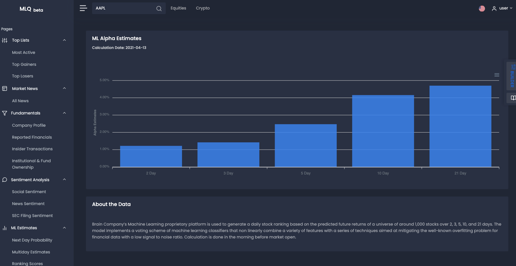
If you want to see how machine learning can be applied to investment research, check out the MLQ app.
The platform combines fundamentals, alternative data, and ML-based insights for smarter trading and investing.
For example, the platform applies machine learning to generate a daily stock ranking based on the predicted future returns of a universe of around 1,000 stocks over 2, 3, 5, 10, and 21 days.
In particular, the model implements a voting scheme of machine learning classifiers that non-linearly combine a variety of features with a series of techniques aimed at mitigating the overfitting problem for financial data with a low signal to noise ratio.
You can sign up for a free account here or can learn more about the platform here.
Resources:


