

In this article we're going to look at a deep reinforcement learning algorithm that has been outperforming all other models: the Twin Delayed DDPG (TD3) algorithm.
By the end of the article, we'll use the Twin Delayed DDPG algorithm to solve a challenging task in AI: teaching a virtual robot how to walk in 3D.
The interesting part about this deep reinforcement learning algorithm is that it's compatible with continuous action spaces. This is contrasted to a discrete action space, in which the agent has a finite number of actions it can take (i.e. turn left, turn right, go forward).
The following article is based on the course Deep Reinforcement Learning 2.0 and is organized as follows:
1. Fundamentals of Twin Delayed DDPG
- 1.1 What is reinforcement learning?
- 1.2 Q-Learning
- 1.3 Deep Q-Learning
- 1.4 Policy Gradient
- 1.5 Actor-Critic Model
- 1.6 Taxonomy of AI models
2. Theory of Twin Delayed DDPG
- 2.1 Q-Learning Steps
- 2.2 Policy Learning Steps
3. Implementation of Twin Delayed DDPG
If you want to check out the research paper that introduced Twin Delayed DDPG you can find it here: Addressing Function Approximation Error in Actor-Critic Methods.
As for the implementation of the algorithm, you can find the GitHub repository for the paper here: PyTorch implementation of TD3 and DDPG for OpenAI gym tasks.
Stay up to date with AI
1. Fundamentals of Twin Delayed DDPG
To start, let's briefly review reinforcement learning.
1.1 What is Reinforcement Learning?
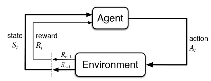
In reinforcement learning, we have an agent that is interacting with an environment.
At every time step, the agent will take as input the State \(S_t\), which represents what's happening in the environment.
The agent then outputs an Action \(A_t\) to perform inside the environment.
As soon as the agent performs the action, the environment returns back a new State \(S_{t+1}\) and the agent receives a Reward \(R_{t+1}\), which lets it know whether it was a good action or not.
Here's how we can visually represent this iterative process:
The goal of an Agent is to maximize its cumulative reward over time.
This is referred to as the return, and more specifically the goal of an agent is to maximize the expected return.
As we'll see, another fundamental principle of reinforcement learning is the policy.
A policy is a function taking as input the state and returning as output the action.
Let's now move onto another fundamental concept in reinforcement learning: Q-Learning.
1.2 Q-Learning
Q-learning is one of the two essential parts of the TD3 model.
As we'll see, the TD3 model actually learns two things at the same time:
- It learns the Q-values, which is based on Q-learning
- And it will learn the parameters of the policy, which are the weights of the policy
In Q-learning the agent learns what are called Q-values, which represent the quality the state and action: Q(state, action).
To understand this, let's look at an example from this Q-learning tutorial.
Suppose we have an agent that needs to cross a maze that has mines in the shortest time possible.
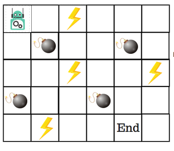
To solve this we make use of a Q-table, which is a lookup table with the maximum expected future rewards for each action in each state.
As we know the goal is the maximize the value function Q.
To do this, at each iteration t >= 1, we repeat the following steps:
- We select a random state \(s_t\) from the possible states
- From that state, we take a random action \(a_t\)
- When we reach the next state \(s_{t+1}\) and we get a reward \(R(s_t, a_t)\)
- We compute the Temporal Difference
- We update the Q-value by applying the Bellman equation
Here's an example of a Q-table:
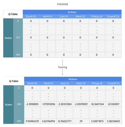
Intuitively, you can think of the Q-table as a cheat sheet for the agent to figure out which action to perform to reach its goal.
But what if the cheat sheet gets too long?
Imagine an environment with 100,000 states and 1000 actions per state...this would create a table with 100 million cells.
Enter deep Q-Learning.
1.3 Deep Q-Learning
Deep Q-learning gets us closer to the TD3 model, as it is said to be the continuous version of deep Q-learning. Deep Q-learning is only applied when we have a discrete action space.
The principle for deep Q-learning is the same as basic Q-learning, except that we have a neural network that learns the Q-values instead of learning them through iterations.
The neural network predicts the Q-values as close to their Q-target as possible.
The way it does this is by computing the loss between the prediction and the target. The goal of the neural network is to reduce the loss over time with backpropagation through stochastic gradient descent.
Here is the process of Deep Q-Learning from this course:
Initialization:
- The memory of the Experience Replay is initialized into an empty list M
- We choose a maximum size of the memory
We then repeat this process at each time step until the end of the epoch:
- We predict the Q-values of the current state
- We take the action with the highest Q-value
- We get the reward
- We reach the next state
- We append the transition in memory
- We take a random batch of transitions. For all transitions of the random batch, we get the predictions and the targets, and then we compute the loss and backpropagate this loss back into the neural network.
Now that we understand deep Q-learning we can move on to the concept of policy gradient, which is the second part that the TD3 model is learning.
1.4 Policy Gradient
As mentioned, policy gradient is the second thing that the TD3 model learns alongside the Q-values.
Policy gradient is a second neural network that consists of updating the weights of the policy. It takes as input the states and outputs actions.
Recall that the return is the sum of the rewards over time, and the goal of the agent is to maximize expected return.
This brings us to policy gradient, as the principle of policy gradient is to compute the gradient of that expected return.
Since we don't actually know what's going to happen in the future (i.e. what reward we'll get), policy gradient is an approximation method.
We then update the parameters \(\phi\) through gradient ascent. We use gradient ascent as opposed to descent because we want to increase the expected return.
To summarize, policy gradient is a technique that directly updates the weights of the policy.
1.5 Actor-Critic
Actor-critic is the model from which TD3 is derived because the actor-critic model is not one single model, instead it is two models working together.
The actor is the policy, which takes as input the states and returns actions as output. The policy can be updated through the deterministic policy gradient algorithm.
The critic takes as input the states and actions concatenated together and returns as output Q-values.
The expected return can be approximated in many ways, and one of them is through the Q-value.
So we're using policy gradient on our critic model which will return and predict Q-values that get closer and closer to a specific target. We use these Q-values to approximate the expected return, which itself is used to perform gradient ascent.
Here's a summary from the TD3 paper:
In actor-critic methods, the policy, known as the actor, can be updated through the deterministic policy gradient algorithm (Silver et al., 2014):
\[∇_\phi J(\phi) =\mathbf{E}_{s∼pπ} [∇_aQ^π (s, a)|_{a=π(s)} ∇_\phiπ_\phi(s)]\]
where \(Qπ (s, a) =\mathbf{E}_{si∼pπ,ai∼π} [Rt|s, a]\), the expected return when performing action a in state s and following π after, is known as the critic or the value function.
1.6 Taxonomy of AI Models
Before we get to the TD3 algorithm, let's review a few important concepts in reinforcement learning.
Model-Free vs. Model-Based
Model-free means the agent is directly taking data from the environment, as opposed to making its own prediction about the environment.
Model-based means the agent learns how to maximize reward by making their own prediction of the environment.
Value-Based vs. Policy-Based
Value-based means the agent is learning to maximize expected reward through learning different values than your parameters, examples of which are Q-learning and deep Q-learning.
Policy-based means that the agent is directly updating the weights of its policy instead of taking an intermediate value such as the Q-value.
Off-Policy vs. On-Policy
Off-policy means the agent can learn from historical data. This is the case when you have an experience replay memory.
On-policy means the agent can only learn on new data, or on new observations.
2. Twin Delayed DDPG (TD3) Theory
Let's now move on to the theory behind the Twin Delayed DDPG model.
As mentioned, DDPG stands for Deep Deterministic Policy Gradient and is a recent breakthrough in AI, particularly in the case of environments with continuous action spaces.
To understand TD3, let's first define why deep Q-learning cannot be applied to continuous action spaces.
Here's the Q-learning algorithm from Wikipedia:
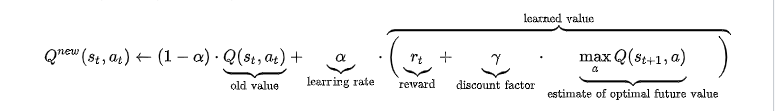
As we can see, the estimate of optimal future values has a maximum term.
In a discrete case, with a finite number of actions, finding this maximum is quite easy.
When you have continuous actions with potentially infinite values, however, finding this maximum becomes a complex optimization task.
This is the reason we don't apply Q-learning to continuous tasks.
To solve this and be able to apply Q-learning to continuous tasks, the authors introduced the Actor-Critic model.
To recap, Actor-Critic has 2 neural networks that the following way:
- The Actor is the policy that takes as input the State and outputs Actions
- The Critic takes as input States and Actions concatenated together and outputs a Q-value
The Critic learns the optimal Q-values which are then used to for gradient ascent to update the parameters of the Actor.
By combining learning the Q-values (which are rewards) and the parameters of the policy at the same time, we can maximize expected reward.
This isn't the optimal solution, however. The research paper describes how there is an approximation error that could be improved, and this is where TD3 comes in.
The first trick to improve the approximation error is to have 2 Critics, instead of one (this is where twin comes from), so each Critic proposes different values of the Q-value.
Let's now break down the Twin-Delayed DDPG algorithm into 15 steps.
2.1 Q-Learning Steps
Step 1: initialize the Replay memory
- Initialize the Experience Replay memory. This will store the past transitions from which it learns the Q-values.
- Each transition is composed of \((s, s', a_1, r_1)\) - the current state, the next state, the action, and the reward.
Step 2: build one neural network for the Actor model and one for the Actor target
- The Actor target is initialized the same as the Actor model, and the weights will be updated over the iterations return optimal actions.
- In terms of the architecture of the neural networks, the authors suggest the following:
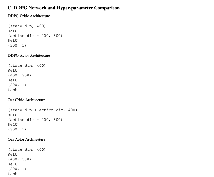
Step 3: build two neural networks for the Critic models and two for the Critic targets.
- We can also see the architecture of these neural networks in the image above. So in total, we have 2 Actor neural networks and 4 Critic neural networks.
- The Actors are learning the Policy, and the Critics are learning the Q-values.
Here's an overview of the training process of these neural networks:
Actor target -> Critic target -> Critic target -> Critic model -> Critic model -> Actor model
- We start by building the Actor targets, which outputs the Actions for the Critic target, which leads to the Critic model, and finally, the Actor model gets its weights updated through gradient ascent.
Now let's move on to the training process.
Step 4: sample a batch of transitions (s, s', a, r) from memory.
- In the implementation, we're going to use 100 batches. The following steps will be done to each transition from the batch (s, s', a, r).
Step 5: from the next state s' the Actor target plays the next action a'
Step 6: add Guassian noise to the next action a' and put the values in a range of values supported by the environment.
- This is to avoid two large actions played from disturbing the state of the environment. The Gaussian noise we're adding is an example of a technique for exploration of the environment. We're adding bias into the action in order to allow the agent to explore different actions.
Step 7: the two Critic targets each takes the couple (s', a') as input and returns two Q-values: \(Q_{t1}(s', a')\) and \(Q_{t2}(s', a')\)
Step 8: keep the minimum of the Q-values: \(min(Q_{t1},Q_{t2})\) - this is the approximated value of the next state.
- Taking the minimum of the two Q-value estimates prevents overly optimistic estimates of the value state, as this was one of the issues with the classic Actor-Critic method.
- This allows us to stabilize the optimization of the Q-learning training process.
Step 9: we use \(min(Q_{t1},Q_{t2})\) to get the final target of the two Critic models:
- The formula for this is \(Q_t = r + \gamma*(min(Q_{t1},Q_{t2}\), where \(\gamma\) is the discount factor.
Step 10: the two Critic models take the couple (s, a) as input and return two Q-values as ouptuts.
- We now compare the minimum Critic target and compare it to the two Q-values from the Critic models: \(Q_1(s, a)\) and \(Q_2(s, a)\).
Step 11: compute the loss between the two Critic models
- The Critic Loss is the sum of the two losses: \(Critic Loss = MSELoss(Q_1(s, a), Q_t) + MSELoss(Q_2(s, a), Q_t)\)
Step 12: backpropagate the Critic loss and update the Critic models parameters.
- We now want to reduce the Critic loss by updating the parameters of the two Critic models over the iterations with backpropagation. We update the weights with stochastic gradient descent with the use of an
Adamoptimizer. - The Q-learning part of the training process is now done, and now we're going to move on to policy learning.
2.2 Policy Learning Steps
Recall that the ultimate goal of the policy learning part of TD3 is to find the optimal parameters of the Actor model (our main policy), in order to perform the optimal actions in each state which will maximize the expected return.
We know that we don't have an explicit formula for the expected return, instead we have a Q-value which is positively correlated with the expected return.
The Q-value is an approximation and the more you increase this value, the closer you get to the optimal expected return.
We're going to use the Q-values from the Critic models to perform gradient ascent by differentiating their output with respect to the weights of the Actor model.
As we update the weights of our Actor model in the direction that increases the Q-value, our agent (or policy) will return better actions that increase the Q-value of the state-action pair, and also get the agent closer to the optimal return.
Step 13: every 2 iterations we update the Actor model by performing gradient ascent on the output of the first Critic model.
- Now the models that haven't been updated yet are the Actor and Critic targets, which leads to the last two steps.
Step 14: every 2 iterations we update the weights of the Actor target with polyak averaging.
- Polyak averaging means that the parameters of the Actor target \(θ'_ i\) are updated by the sum of tao * theta, where tao is a very small number and theta is the parameters of the Actor model.
- The other part is \((1 − τ )θ'_i\), where \(θ'_i\) is the parameters of the Actor target before the update:
\[θ'_ i ← τθ_i + (1 − τ )θ'_i\]
- This equation represents a slight transfer of weights from the Actor model to the Actor target. This makes the Actor target get closer and closer to the Actor model with each iteration.
- This gives time to the Actor model to learn from the Actor target, which stabilizes the overall learning process.
Step 15: once every two iterations we update the weights of the Critic target with polyak averaging.
- The equation for updating the weights is the same here:
\[\phi' ← τ\phi + (1 − τ )\phi'\]
- The one step that we haven't covered yet is the delayed part of the algorithm.
- The delayed part of the model comes from the fact that we're updating the Actor and the Critic once every two iterations. This is a trick to improve performance with respect to the classical version of DDPG.
3. Implementation of Twin-Delayed DDPG
We won't go into detail about the implementation in this article, but you can check out this GitHub for the PyTorch implementation.
Instead, here are the results we see after running the code from the Deep Reinforcement Learning 2.0 course.
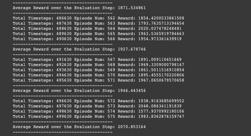
We'll implement the code for the ant - a continuous 3D environment, and the training process will run for 500,000 timesteps.
Ant Implementation:
The ant environment is the most challenging of the three since it is in 3-dimensions. As we can see below we achieve a reward over 2000 in the final timesteps, an incredible feat!
4. Summary of Twin Delayed DDPG
To summarize, in this article we looked at a deep reinforcement learning algorithm called the Twin Delayed DDPG model.
The interesting thing about this algorithm is that it can be applied to continuous action spaces, which are very useful for many real-world tasks.
We first looked at the fundamentals of the TD3 algorithm, which include:
- Q-learning
- Deep Q-learning
- Policy gradient
- Actor-Critic model
We then moved on to the theory of the TD3 algorithm, which includes 15 steps to train our model.
Finally, we implemented the training process of 500,000 timesteps for the 3D continuous act of teaching an ant to walk with incredible results.


