

In our previous articles in this series, we've downloaded our historical bitcoin data, build, built a naive forecasting model as a baseline, and created a function to evaluate our models with several common evaluation metrics.
We're almost ready to start building models, although first we need to do some more data preprocessing.
In this article, we're going to format our time series data with windows and horizons. We'll discuss why this is useful in more detail later, but in short, windows allow us to turn forecasting into a supervised learning problem.
This article is based on notes from this TensorFlow Developer Certificate course and is organized as follows:
- Windowing our dataset
- Sliding windows vs. expanding windows
- Writing a function to turn time series data into windows and labels
- Turning our windowed data into training and test sets
Previous articles in this series can be found below:
- Time Series with TensorFlow: Downloading & Formatting Historical Bitcoin Data
- Time Series with TensorFlow: Building a Naive Forecasting Model
- Time Series with TensorFlow: Common Evaluation Metrics
Stay up to date with AI
Windowing our dataset
As mentioned, the reason we want to window our time series dataset is to turn forecasting into a supervised learning problem.
To recap, here are two terms to be familiar with:
- Horizon: The number of timesteps into the future we want to predict
- Window size: The number of timesteps we're going to use to predict the horizon.
Before we write code, let's write some pseudo-code—say we want to window our data for one week and predict the next day as follows:
[0, 1,  2, 3, 4, 5, 6] -> [7]
[1,  2, 3, 4, 5, 6, 7] -> [8]
[2,  3, 4, 5, 6, 7, 8] -> [9]
Right now our data y_train is one big array of examples (prices) with a length of 2356. We also have the variable btc_price that we want to turn into windows.
If we wanted just the first 7 days of the dataset for the window and the 8th day as the horizon, we could just do this:
print(f"We want to use {btc_price[:7]} to predict this {btc_price[7]}")We now want to create a function that will do this for us for any time period.
First, let's setup global variables for window and horizon size:
# global variables for window and horizon size
HORIZON = 1
WINDOW_SIZE = 7
Next, we'll create a function to label windowed data:
# Create a function to label windowed data
def get_labelled_window(x, horizon=HORIZON):
  """
  Create labels for windowed dataset
  E.g if horizon = 1
  Input: [0, 1,  2, 3, 4, 5, 6, 7] -> Output: ([0, 1,  2, 3, 4, 5, 6], [7])
  """
  return x[:, :-horizon], x[:, -horizon]
Let's test out the new function:
# Test our window labelling function
test_window, test_label = get_labelled_window(tf.expand_dims(tf.range(8), axis=0))
print(f"Window: {tf.squeeze(test_window).numpy()} -> Label: {tf.squeeze(test_label).numpy()}")
Window: [0 1 2 3 4 5 6] -> Label: 7
We now have a starting point for a windowing function, although it only works on one input (i.e. [0 1 2 3 4 5 6]).
We now need to scale this up across our entire BTC price array.
Sliding windows vs. expanding windows
There are two major approaches to test forecasting models, namely the sliding window and expanding window. As Uber highlights:
In the sliding window approach, one uses a fixed size window, shown here in black, for training. Subsequently, the method is tested against the data shown in orange.
On the other hand, the expanding window approach uses more and more training data, while keeping the testing window size fixed.
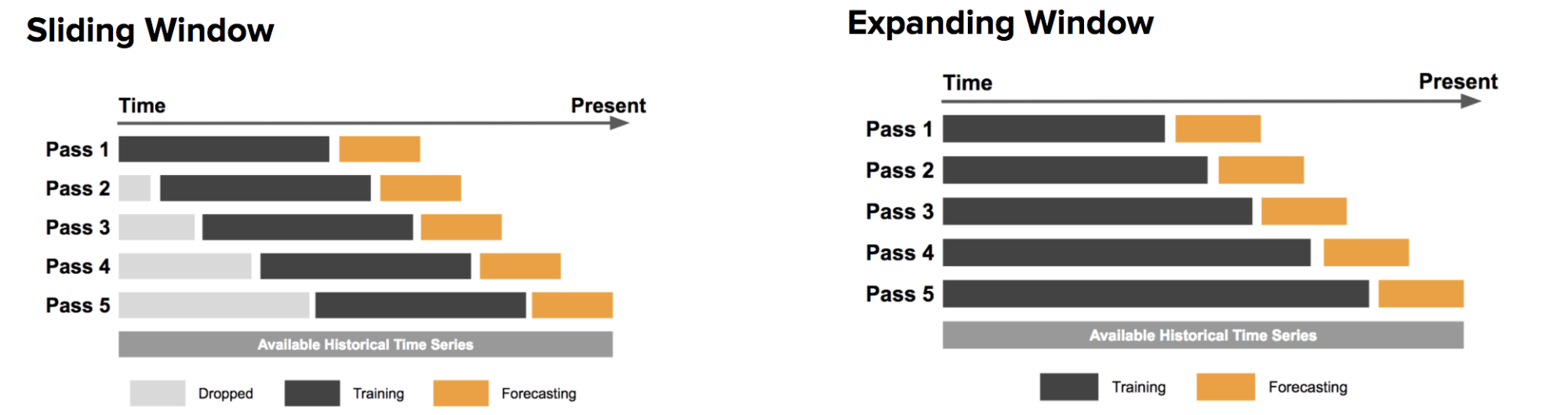
In this project, we're going to focus on the sliding window approach.
Writing a function to turn time series data into windows and labels
As mentioned, we have a way to label our windowed data on a small scale, but we need a way to do this across our entire time series dataset.
We could do this with Python for loops, but for large datasets, this would be quite slow. To speed this up, we'll use NumPy's array indexing.
The steps our function needs to take include:
- Create a window step of specific window size (i.e. [0, 1, 2, 3, 4, 5, 6])
- Use NumPy indexing to create a 2D array of multiple window steps, for example: [0, 1, 2, 3, 4, 5, 6], [1, 2, 3, 4, 5, 6, 7], [ 2, 3, 4, 5, 6, 7, 8]
- Use the 2D array of multiple window steps (from 2) to index on a target series (e.g. historical price of Bitcoin)
- Use our
get_labelled_window()function we created to turn the window steps into windows with a specified horizon
The function below has been adapted from this blog post: Fast and Robust Sliding Window Vectorization with NumPy.
To break this up, let's do the first two steps and then visualize the window indexes as follows:
# Create a function to view NumPy arrays as windows
def make_windows(x, window_size=WINDOW_SIZE, horizon=HORIZON):
  """
  Turns a 1D array into a 2D array of sequential labelled windows of window_size with horizon size label.
  """
  # 1. Create a window of specific window_size (add the horizon on the end for labelling later)
  window_step = np.expand_dims(np.arange(window_size+horizon), axis=0)

  # 2. Create a 2D array of multiple window steps (minus 1 to account for 0 indexing)
  window_indexes = window_step + np.expand_dims(np.arange(len(x)-(window_size+horizon-1)), axis=0).T # create 2D array of windows of window size

  print(f"Window indexex:\n {window_indexes, window_indexes.shape}")
make_windows(prices, window_size=WINDOW_SIZE, horizon=HORIZON)Window indexex:
(array([[ 0, 1, 2, ..., 5, 6, 7],
[ 1, 2, 3, ..., 6, 7, 8],
[ 2, 3, 4, ..., 7, 8, 9],
...,
[2935, 2936, 2937, ..., 2940, 2941, 2942],
[2936, 2937, 2938, ..., 2941, 2942, 2943],
[2937, 2938, 2939, ..., 2942, 2943, 2944]]), (2938, 8))Let's continue on with step 3 and 4 and complete our function as follows:
# Create a function to view NumPy arrays as windows
def make_windows(x, window_size=WINDOW_SIZE, horizon=HORIZON):
  """
  Turns a 1D array into a 2D array of sequential labelled windows of window_size with horizon size label.
  """
  # 1. Create a window of specific window_size (add the horizon on the end for labelling later)
  window_step = np.expand_dims(np.arange(window_size+horizon), axis=0)

  # 2. Create a 2D array of multiple window steps (minus 1 to account for 0 indexing)
  window_indexes = window_step + np.expand_dims(np.arange(len(x)-(window_size+horizon-1)), axis=0).T # create 2D array of windows of window size
  print(f"Window indexex:\n {window_indexes, window_indexes.shape}")

  # 3. Index on the target array with 2D array of multiple window sets
  windowed_array = x[window_indexes]

  #4. Get the labelled windows
  windows, labels = get_labelled_window(windowed_array, horizon=horizon)
  return windows, labels
Let's make sure the function works and pass the full labels and full windows of the prices array:
full_windows, full_labels = make_windows(prices, window_size=WINDOW_SIZE, horizon=HORIZON)Let's take a look at the first few windows & labels
# View the first 3 windows & labels
for i in range(3):
  print(f"Window: {full_windows[i]} -> Label: {full_labels[i]}")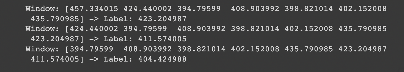
To summarize, we've now got a preprocessing function that will take in a set of training data and a label to try and predict.
We've turned our data from a time series — i.e. a single array of variables — into a supervised learning problem.
Now that we've done this ourselves, it's important to note that there's a function in Keras that does the same thing: it takes in an array and returns a windowed dataset: tf.keras.utils.timeseries_dataset_from_array()
This function also has the benefit of returning data in the form of a tf.data.Dataset instance.
Turning our windowed data into training and test sets
The final step before we can start building models is turning our windowed time series data into training and test sets.
If you recall in a previous article, we created a function to split the entire dataset into train and test sets, we now just need to do this for our windowed data.
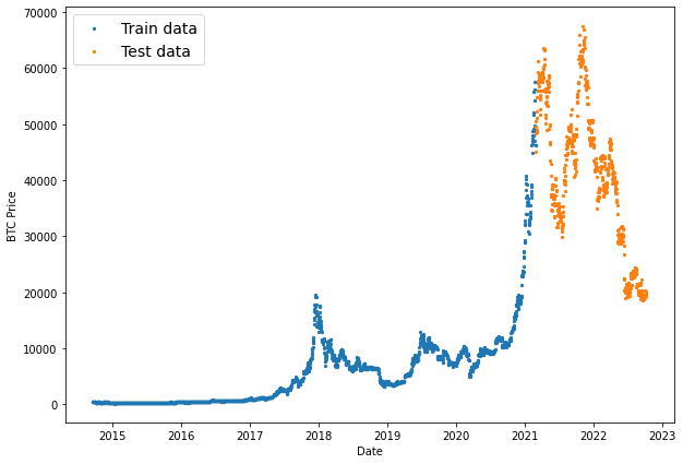
Since we already have full_windows and full_labels, we just need to split these up into train and test sets using indexing as follows:
# Make train/test splits
def make_train_test_splits(windows, labels, test_split=0.2):
  """
  Splits matching pairs of windows and labels into train and test splits.
  """
  split_size = int(len(windows) * (1-test_split)) # this will default to 80% train, 20% test
  train_windows = windows[:split_size]
  train_labels = labels[:split_size]
  train_windows = windows[split_size:]
  train_labels = labels[split_size:]
  return train_windows, test_windows, test_windows, test_labels
Let's test it out and create train and test windows:
# Create train and test windows
train_windows, test_windows, train_labels, test_labels = make_train_test_splits(full_windows, full_labels)
len(train_windows), len(test_windows), len(train_labels), len(test_labels)
(2350, 588, 2350, 588)
We now have train and test splits for our windowed data, it's time to start building a few models.
Summary: Formatting Data with Windows & Horizons
In this article, we created a function to format our data as a sliding window.
The reason we want to use windows and labels is so we can turn forecasting into a supervised learning problem.
Finally, we turned our windowed time series data into training and test sets.
In this next article, we'll create a modeling checkpoint callback to save our best performing model and create our first deep learning models for time series forecasting.


