In this article we're going to cover an important concept in machine learning: transfer learning.
The following article is based on notes from this course on TensorFlow 2.0 Practical Advanced and is organized as follows:
- What is Transfer Learning?
- The Transfer Learning Process
- Transfer Learning Strategies & Advantages
- Transfer Learning: Problem Statement
- Evaluate the Model
What is Transfer Learning?
Transfer learning is a machine learning technique in which a network that has already been trained to perform a specific task is repurposed as a starting point for another similar task.
Transfer learning is essentially transferring knowledge from one network to another so that you don't have to start from scratch when it comes to training a model.
The reason that transfer learning is so powerful is that since our starting point is a pre-trained model, this can drastically reduce the computational time needed for training.
As you know from growing up as a baby and having to learn how walk, how to speak, how to write, these things take years of accumulated knowledge and experience to learn. What we can do with transfer learning is skip this learning period and just tweak the new model to fit our specific task.
To do this, in transfer learning we start with a base Artificial Neural Network that has already been trained. We don't actually take the entire model, but instead just take the trained network weights and we try to repurpose it to a second ANN that can perform a new function on a new dataset.
As you can imagine, transfer learning works very well if the features are general in nature so that the trained weights can effectively be repurposed.
Stay up to date with AI
The Transfer Learning Process
To understand the transfer learning process, let's say we want to train a convolutional neural network on the ImageNet dataset.
To do this we can apply a convolutional layer with kernels and feature detectors in the first two layers. We can then flatten our feature maps and feed it to a fully-connected artificial neural network.
Let's assume that our CNN has been trained to classify three classes of animals including elephants, snakes, and lions.
With transfer learning we can take the first two convolutional layers and take the weights and copy them to another neural network.
We can then use new images that are not in the ImageNet dataset, for example we could have a new dataset with images of cats and dogs. We're not going to take the fully-connected dense layer from the first network, instead we're going to introduce a new dense layer architecture, we initialize it randomly, and then we start our training process.
The reason we take the first CNN layers and not the dense network is that these layers are used to extract high level general features. The last few layers are custom because we're using them to learn and perform classification on a new specific task.
Transfer Learning Strategies & Advantages
There two transfer learning strategies we're going to cover, which are widely used in machine learning, these include:
Strategy 1
- Freeze the trained CNN network weights from the first layers
- Only train the newly added dense layers, which are created from randomly initializing the weights
Strategy 2
- Initialize the CNN network with the pre-trained weights
- We then retrain the entire CNN network while setting the learning rate to be very small, which ensures that we don't drastically change the trained weights
As mentioned, the advantage of transfer learning is that it provides fast training progress since we're not starting from scratch. Transfer learning is also very useful when you have a small training dataset available, but there's a large dataset in a similar domain (i.e. ImageNet).
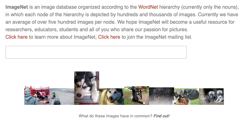
ImageNet
The dataset that we will use for transfer learning is called ImageNet, which is an open source repository of images that consist of 1000 classes and over 1.5 million images.
Transfer Learning: Problem Statement
In this practical example of transfer learning we're going to repurpose trained weights from the ResNet 50, which is a famous deep neural network, to perform classification on a new dataset.
This model has been trained on ImageNet, and we're going to repurpose it to classify new images of cats and dogs.
The new model we'll create will consist of a base pre-trained network and a new dense network classifier. The feature maps that were previously trained will be augmented with a new dense layers.
As mentioned, the first step is to freeze the layers we obtained from the pre-trained model and only train the final classifier layer.
After that, we can do some fine tuning by unfreezing the base layers and slowly training it with a low learning rate so the entire network's performance can be improved.
The first step in Google Colab is to !pip install tensorflow-gpu==2.0.0.alpha0.
Next we need to import the following packages:
import tensorflow as tf
import pandas as pd
import numpy as np
import matplotlib.pyplot as plt
import seaborn as sns
import random
Import the Model
Now we need to import the ResNet 50 model using keras, and we need to specify that the model is trained with the ImageNet weights:
model = tf.keras.applications.ResNet50(weights='imagenet')
Apply Transfer Learning & Retrain the Model
Now that we've downloaded the model let's apply transfer learning and retrain the model on a new dataset.
Recall that we're going to build our new model with two pieces:
- The base network, which comes from ResNet 50 and is already trained
- In the code below you can see we use
include_top = False, which means we don't want to include the end of the network so we can add our own classifier
base_model = tf.keras.applications.ResNet50(weights='imagenet', include_top = False)
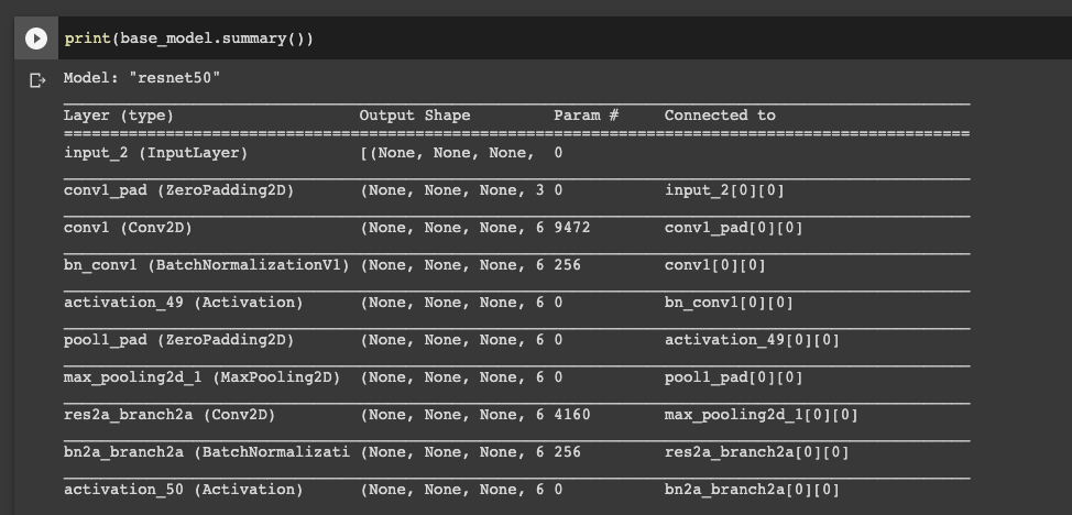
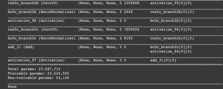
print(base_model.summary())
Here we can see this is a massive network with millions of trainable parameters:
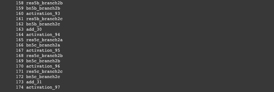
Now let's visualize the various layers with a for loop, and you can see that we have 174 layers with different names:
for i, layer in enumerate(base_model.layers):
  print(i, layer.name)
Now we're ready to take the base model and perform transfer learning with a new classification task.
The first step is to take the output from the base model and perform GlobalAveragePooling2D(), which will condense our feature maps from the output and then we'll add our dense fully connected artificial neural network at the end:
x = base_model.output
x = tf.keras.layers.GlobalAveragePooling2D()(x)
x = tf.keras.layers.Dense(1024, activation='relu')(x)
x = tf.keras.layers.Dense(1024, activation='relu')(x)
x = tf.keras.layers.Dense(1024, activation='relu')(x)
x = tf.keras.layers.Dense(512, activation='relu')(x)
preds = tf.keras.layers.Dense(2, activation ='softmax')(x)We can see that the final layer has 2 neurons as the output since we're classifying cats and dogs. Now we're ready to create our own network, which consists of the base model and the output, which is our preds:
model = tf.keras.models.Model(inputs=base_model.input, outputs=preds)
print(model.summary())
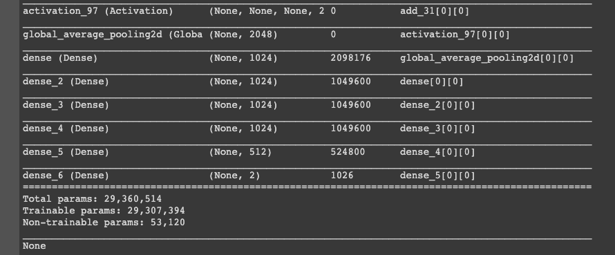
Now we can see we have the same network as before, but after the last layer we've added our GlobalAveragePooling2D() layer and our fully connected dense layers.
If we print the layer names again we can see we now have 180 layers:
for i, layer in enumerate(model.layers):
  print(i, layer.name)
What we're going to do next is freeze the layers that have already been trained, so all the layers up until layer 174:
for layer in model.layers[:175]:
  layer.trainable = False
Then for layer 175 and up we want these layers to be trainable:
for layer in model.layers[175:]:
  layer.trainable = True
Now we're going to use our new data and apply a preprocessing function:
train_datagen = tf.keras.preprocessing.image.ImageDataGenerator(preprocessing_function=tf.keras.applications.resnet50.preprocess_input)Next we're going to take the images from our directory in batches and categorical classes:
train_generator = train_datagen.flow_from_directory('/content/drive/My Drive/Colab Notebooks/TF 2.0 Advanced/Transfer Learning Data/train/',
                                                   target_size = (224, 224),
                                                   color_mode = 'rgb',
                                                   batch_size = 32,
                                                   class_mode = 'categorical',
                                                   shuffle = True)
We can see there are 202 images and 2 classes. Now we want to compile our model, fit our model with model.fit_generator, and then train it on 5 epochs:
model.compile(optimizer='Adam', loss='categorical_crossentropy', metrics=['accuracy'])history = model.fit_generator(generator = train_generator, steps_per_epoch=train_generator.n//train_generator.batch_size, epochs = 5)We can see with just 5 epochs we can get nearly 98% accuracy:

Evaluate the Model
Let's now evaluate the model that we just trained. The first step to do this is to plot the performance of the model in terms of accuracy and loss.
acc = history.history['accuracy']
loss = history.history['loss']

plt.figure()
plt.plot(acc, label='Training Accuracy')
plt.ylabel('Accuracy')
plt.title('Training Accuracy')

plt.figure()

plt.plot(loss, label='Training Loss')
plt.ylabel('Loss')
plt.title('Training Loss')
plt.xlabel('epoch')
plt.show()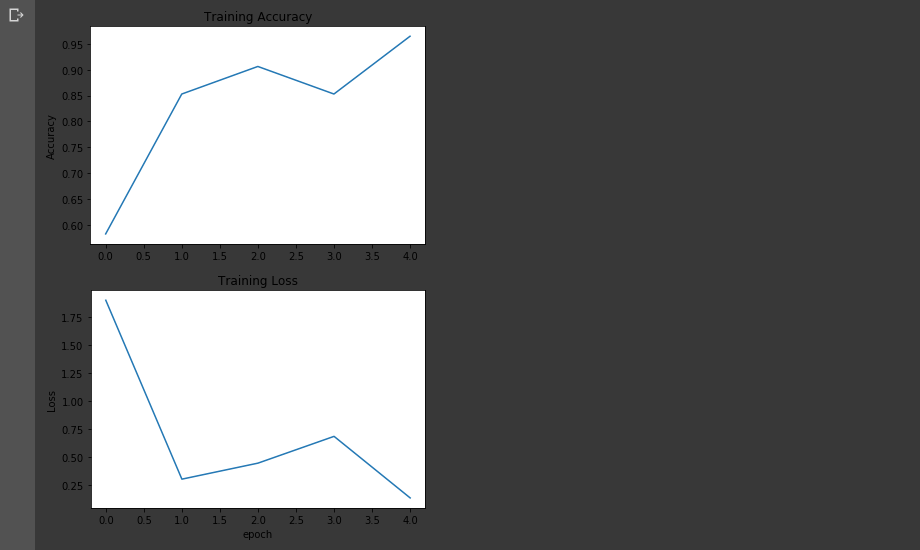
We can see that with transfer learning in one epoch we get almost 90% accuracy. Now let's load two images from the new dataset and test the model.
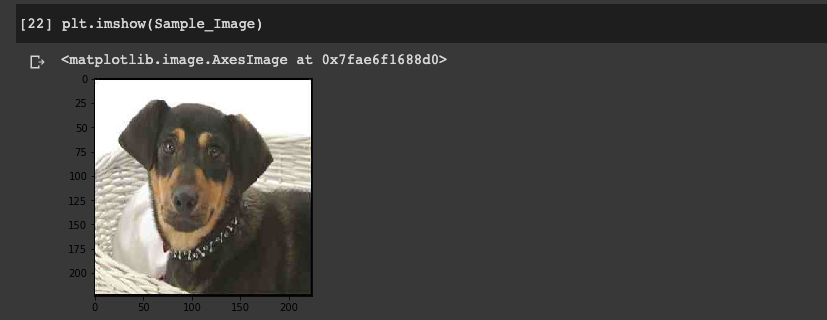
Before we test the model we need to convert the image to an array:
Sample_Image = tf.keras.preprocessing.image.img_to_array(Sample_Image)Next we need to expand the dimensions and then we can use the model for prediction:
Sample_Image = np.expand_dims(Sample_Image, axis = 0)
Sample_Image = tf.keras.applications.resnet50.preprocess_input(Sample_Image)
predictions = model.predict(Sample_Image)
print('Predictions:', predictions)
Predictions: [[0.03529738 0.9647026 ]]
For the prediction the left number is for cat and the right number is for dogs, and we can see the model predicts a 96% probability that this image is a dog.
Summary: Transfer Learning with TensorFlow 2.0
As we've seen, transfer learning is a very powerful machine learning technique in which we repurpose a pre-trained network to solve a new task.
Since we're transferring knowledge from one network to another and don't have to start from scratch, this means that we can drastically reduce the computational power needed for training. In particular, we saw that with just 5 epochs we were able to get a high degree of accuracy for our model with a completely new dataset.


